Last week I finished preparing new teaching material for a workshop on R optimization techniques. Some of the examples were motivated by benchmarking tests I ran on data manipulation methods with base vs dplyr vs data.table.
Not surprisingly, data.table was generally most efficient in terms of speed when running the microbenchmark tests.
One oddball result did creep up …
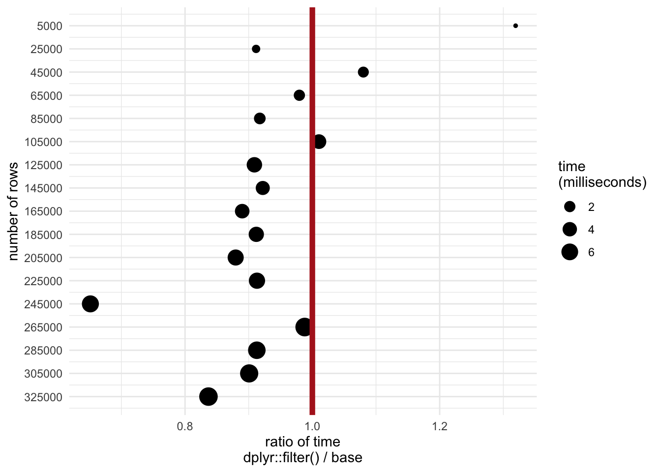
When comparing dplyr::filter() versus a base method (using bracket indices and which()), I noticed that the former was quite a bit slower for a data frame with 5000 rows. But that result reversed as the size of the data frame increased … in other words, filter() was actually much faster for a larger dataset.
First we can load the packages we’ll be using:
library(microbenchmark)
library(dplyr)
library(ggplot2)
library(nycflights13)
Next create a sample of n = 5000 rows of the nycflights13 dataset:
flights_sample <-
  sample_n(flights, 5000)
Then run the benchmark on the sample of n = 5000 rows:
# run benchmark on n = 5000
microbenchmark(
  bracket = flights_sample[which(flights_sample$dep_delay > 0),],
  filter = filter(flights_sample, dep_delay > 0),
  times = 10
  )
## Unit: microseconds
## expr min lq mean median uq max neval
## bracket 223.183 246.329 310.3268 290.7345 315.310 632.726 10
## filter 265.342 352.911 387.6371 371.1365 382.088 673.066 10Now run the benchmark on the full n = 336776 rows:
microbenchmark(
  bracket = flights[which(flights$dep_delay > 0),],
  filter = filter(flights, dep_delay > 0),
  times = 10
  )
## Unit: milliseconds
## expr min lq mean median uq max neval
## bracket 8.844108 9.041099 12.35393 12.58248 13.52227 20.33769 10
## filter 8.001824 8.159017 12.65863 12.27404 13.27080 21.73494 10My guess is that there’s some overhead to using filter() … but this clearly pays off eventually. So how big (i.e. how many rows) does a data frame need to be for filter() to be faster?
# create sequence of number of rows to sample by 20000
sample_seq <- seq(5000, nrow(flights), by = 20000)

# set up empty data frame that will store results
mbm <- data_frame()

# loop through the samples and calculate microbencharmk in ms
for(n in sample_seq) {

  flights_sample <- sample_n(flights, n)

  tmpmbm <-
    microbenchmark(
      bracket = flights_sample[which(flights_sample$dep_delay > 0),],
      filter = filter(flights_sample, dep_delay > 0),
      times = 10,
      unit = "ms"
    )

  mbm <- rbind(mbm, summary(tmpmbm))

}

# add the sample n as a column for plotting
mbm$n <- rep(sample_seq, each = 2)
The plot below shows the threshold (number of rows on y axis) at which filter() is faster (ratio < 1 on x axis). It also demonstrates that the absolute amount of time starts leveling off as the datasets get bigger.
mbm %>%
  select(method = expr,
         nrows = n,
         time = median) %>%
  group_by(nrows) %>%
  mutate(ratio = time / lag(time)) %>%
  filter(!is.na(ratio)) %>%
  ggplot(aes(nrows, ratio, size = time)) +
  geom_point() +
  geom_hline(yintercept = 1, col = "firebrick", lwd = 2) +
  scale_x_reverse(breaks = sample_seq) +
  xlab("number of rows") +
  ylab("ratio of time\ndplyr::filter() / base") +
  coord_flip() +
  theme_minimal() +
  guides(size = guide_legend(title = "time\n(milliseconds)"))