Circular Barplots

Jun 16, 2019 4 min read notes

While preparing figures for a manuscript recently, the first author proposed a plot to compare several phenotypes from every donor in the study. One suggestion was a series of circular barplots (normalized since each phenotype was on a different scale) side-by-side.

Using ggplot2 that might look something like this:

library(ggplot2)
library(tidyr)
library(dplyr)

msleep %>%
  select(name,sleep_total,brainwt,bodywt) %>%
  filter(complete.cases(.)) %>%
  gather(key,value, -name) %>%
  group_by(key) %>%
  mutate(value = percent_rank(value)) %>%
  ggplot(aes(name,value)) +
  geom_col() +
  coord_polar() +
  facet_wrap(~ key, ncol = 3) +
  labs(x = NULL,
       y = "Percentile") +
  theme_minimal()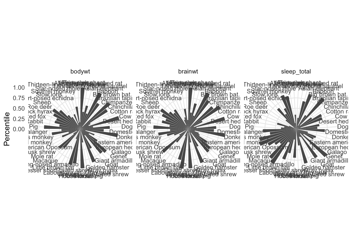

The figure isn’t easy to interpret in this configuration. Even if the canvases of each of the facets were bigger, the labels would need to be rotated for legibility. With that done, it may still be hard to visually connect phenotypes across individuals. In this example, you have to squint at all three facets consecutively, and even do some jumping back and forth. Eventually you may see that some of the largest animals (in terms of both brain and body weight) actually rank quite low in terms of total sleep … and vice versa.

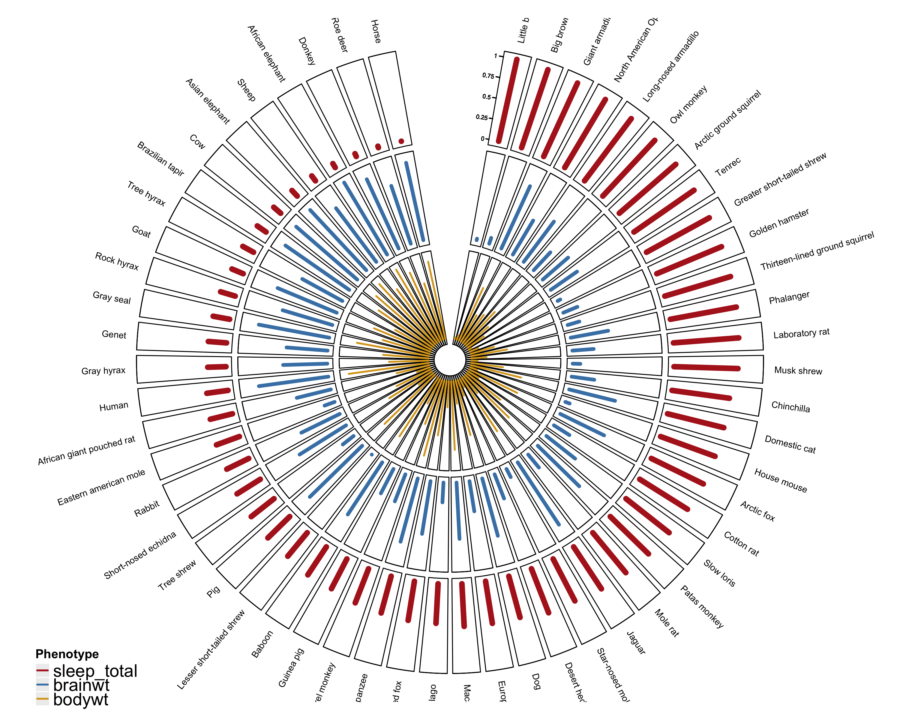
One alternative is to plot the bars as concentric circles, with the bars for phenotypes lined up at each individual.

This is where I stepped away from ggplot2 and started using the circlize package. The syntax took some getting used to … but overall I found the package to be quite useful. There was plenty of documentation in the circlize book. And I was able to build on some of the examples to get where I needed to go:

library(circlize)
library(ComplexHeatmap)
library(gridBase)
library(ggplot2)
library(tidyr)
library(dplyr)

sleep_size <-
  msleep %>%
  select(name,sleep_total,brainwt,bodywt) %>%
  filter(complete.cases(.)) %>%
  mutate(sleep_total = percent_rank(sleep_total),
         brainwt = percent_rank(brainwt),
         bodywt = percent_rank(bodywt),
         index = 1) %>%
  arrange(desc(sleep_total)) %>%
  mutate(name = factor(name))

sleep_size$name <- factor(sleep_size$name, 
                          levels = as.character(sleep_size$name))

# barplot colors
barcols  <- c("firebrick","steelblue","goldenrod")

# parameters for each of the concentric plots
circos.par(cell.padding = c(0.02, 0, 0.02, 0),
           gap.after = c(rep(1, nrow(sleep_size)-1), 20),
           start.degree = 80,
           track.height = 0.3)

# initialize
# at each level of the factor (in this case animal name) plot at index (x=1 for all animals)
# make sure the limit is set to give room one either side of x for each plot
circos.initialize(factors = sleep_size$name, 
                  x = sleep_size$index, 
                  xlim = c(0,2))

# create "track" region for and add lines for with y values for scaled sleep total
circos.trackPlotRegion(factors = sleep_size$name, 
                       y = sleep_size$sleep_total, 
                       panel.fun = function(x, y) {
  
  name = get.cell.meta.data("sector.index")
  i = get.cell.meta.data("sector.numeric.index")
  xlim = get.cell.meta.data("xlim")
  ylim = get.cell.meta.data("ylim")
  
  #text direction (dd) and adjusmtents (aa)
  theta = circlize(mean(xlim), 1.3)[1, 1] %% 360
  dd <- ifelse(theta < 90 || theta > 270, "clockwise", "reverse.clockwise")
  aa = c(1, 0.5)
  if(theta < 90 || theta > 270)  aa = c(0, 0.5)
  
  #plot country labels
  circos.text(x=mean(xlim), y=1.2, labels=name, facing = dd, cex=0.6,  adj = aa)
  
  #plot main sector
  
  circos.axis(labels=FALSE, major.tick=FALSE)
  circos.yaxis(side = "left", at = seq(0, 1, by = 0.25),
               sector.index = get.all.sector.index()[1], labels.cex = 0.4, labels.niceFacing = FALSE)
  
})

circos.trackLines(factors = sleep_size$name, 
                  x = sleep_size$index, 
                  y = sleep_size$sleep_total, 
                  pch=20, 
                  cex=2, 
                  col = barcols[1],
                  type="h", 
                  lwd = 6)

# ... same as above but for body weight
circos.trackPlotRegion(factors = sleep_size$name, 
                       y = sleep_size$bodywt, 
                       panel.fun = function(x, y) {
                         
  circos.axis(labels=FALSE, major.tick=FALSE)
                         
})

circos.trackLines(factors = sleep_size$name, 
                  x = sleep_size$index, 
                  y = sleep_size$bodywt, 
                  pch=20, 
                  cex=2, 
                  col = barcols[2],
                  type="h", 
                  lwd = 4)

# ... same as above but for brain weight
circos.trackPlotRegion(factors = sleep_size$name, 
                       y = sleep_size$brainwt, 
                       panel.fun = function(x, y) {
                         
  circos.axis(labels=FALSE, major.tick=FALSE)
                         
})

circos.trackLines(factors = sleep_size$name, 
                  x = sleep_size$index, 
                  y = sleep_size$brainwt, 
                  pch=20, 
                  cex=2, 
                  col = barcols[3],
                  type="h", 
                  lwd = 2)

circos.clear()

# add legend using complex heatmap
# http://jokergoo.github.io/blog/html/add_legend_to_circlize.html
lgd_lines = Legend(at = colnames(sleep_size)[2:4],
                   type = "lines",
                   legend_gp = gpar(col = barcols, lwd = 2),
                   title_position = "topleft",
                   labels_gp = gpar(fontsize = 14, lex = 4),
                   title = "Phenotype")

lgd_list_vertical = packLegend(lgd_lines)


pushViewport(viewport(x = unit(10, "mm"), y = unit(4, "mm"),
                      width = grobWidth(lgd_list_vertical),
                      height = grobHeight(lgd_list_vertical),
                      just = c("left", "bottom")))

grid.draw(lgd_list_vertical)
upViewport()

circlize R ggplot2

Circular Barplots

Related